<출처>
- 책 : 혼자 공부하는 머신러닝 + 딥러닝
- 저자 : 박해선
- 예제 : https://github.com/rickiepark/hg-mldl / 3-2장
GitHub - rickiepark/hg-mldl: <혼자 공부하는 머신러닝+딥러닝>의 코드 저장소입니다.
<혼자 공부하는 머신러닝+딥러닝>의 코드 저장소입니다. Contribute to rickiepark/hg-mldl development by creating an account on GitHub.
github.com
- 이전 포스팅 이어서~
2023.07.18 - [데이터분석] - [23.07.18] 머신러닝(k-최근접 이웃 회귀) - 33(2)
[23.07.18] 머신러닝(k-최근접 이웃 회귀) - 33(2)
책 : 혼자 공부하는 머신러닝 + 딥러닝 저자 : 박해선 예제 : https://github.com/rickiepark/hg-mldl 1. scikit-learn 1) KNeighborsRegressor - k-최근접 이웃 회귀 모델을 만드는 사이킷런 클래스 - n_neighbors 매개변수로
gmwoo.tistory.com
<핵심 패키지 및 함수>
1. scikit-learn
1) KNeighborsRegressor
- k-최근접 이웃 회귀 모델을 만드는 사이킷런 클래스
<시작하기 전에>
- 이전 포스팅 모델을 사용하여 길이가 50cm인 농어의 무게를 예측했을 때
- 1033g 정도로 예측 -> 하지만 실제 농어의 무게는 훨씬 더 나간다고 함(오류 발생)
print(knr.predict([[50]]))
# 출력 : [1033.33333333]
- 이를 시각화 하면,
import matplotlib.pyplot as plt
# 50cm 농어의 이웃을 구합니다
distances, indexes = knr.kneighbors([[50]])

# 훈련 세트의 산점도를 그립니다
plt.scatter(train_input, train_target)
# 훈련 세트 중에서 이웃 샘플만 다시 그립니다
plt.scatter(train_input[indexes], train_target[indexes], marker='D')
# 50cm 농어 데이터
plt.scatter(50, 1033, marker='^')
plt.xlabel('length')
plt.ylabel('weight')
plt.show()
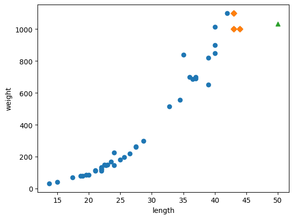
- 이웃 샘플(n_neighbors=3, 총 3개) 타깃의 값 하나를 출력 후 평균을 구해보면,
print(knr.predict([[100]]))
[1033.33333333]
print(np.mean(train_target[indexes]))
1033.3333333333333
- k-최근접 이웃 회귀는 가장 가까운 샘플을 찾아 타깃을 평균하므로 새로운 데이터가 훈련 세트의 범위를 벗어나면 엉뚱한 값을 예측할 수 있음 (예로, 100cm인 농어도 여전히 1033g으로 예측하게 됨)
# 100cm 농어의 이웃을 구합니다
distances, indexes = knr.kneighbors([[100]])

# 훈련 세트의 산점도를 그립니다
plt.scatter(train_input, train_target)
# 훈련 세트 중에서 이웃 샘플만 다시 그립니다
plt.scatter(train_input[indexes], train_target[indexes], marker='D')
# 100cm 농어 데이터
plt.scatter(100, 1033, marker='^')
plt.xlabel('length')
plt.ylabel('weight')
plt.show()
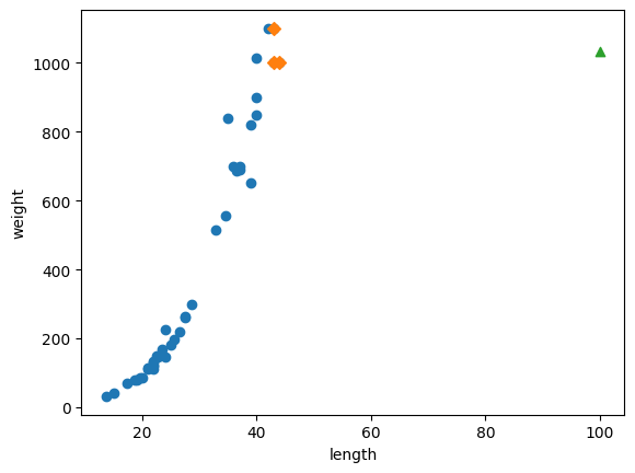
따라서 새로운 알고리즘이 필요 !
<선형 회귀>
1. Linear regression
1) 개념
- 대표적인 회귀 알고리즘이며, 간단하고 성능이 뛰어남
- 특성이 하나인 경우 어떤 직선을 학습하는 알고리즘
2) LinearRegression()
from sklearn.linear_model import LinearRegression
lr = LinearRegression()
# 선형 회귀 모델 훈련
lr.fit(train_input, train_target)
LinearRegression()On GitHub, the HTML representation is unable to render, please try loading this page with nbviewer.org.
- y = a*x + b
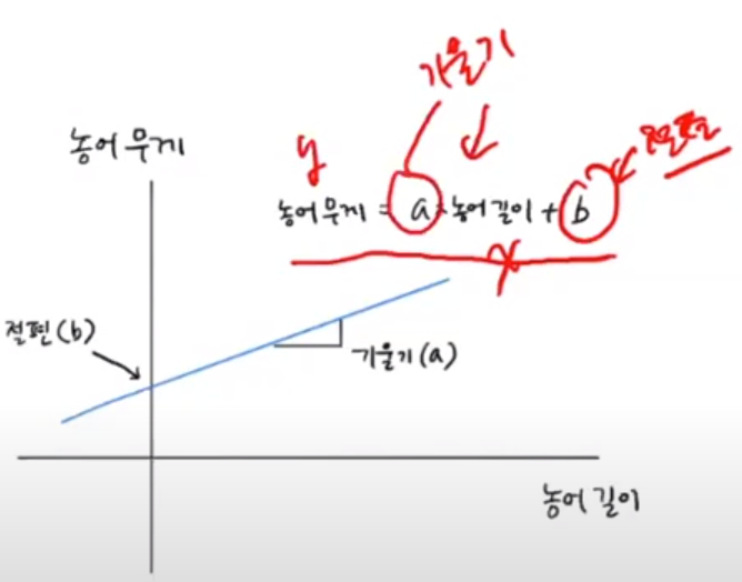
- 모델 파라미터 -> coef_ : 기울기 , intercept_ : 절편
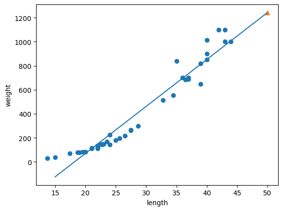
print(lr.coef_, lr.intercept_)
[39.01714496] -709.0186449535477
- 50cm 농어에 대한 예측을 해보면, 1241g으로 더 알맞은 결과가 나옴
# 50cm 농어에 대한 예측
print(lr.predict([[50]]))
[1241.83860323]
- 하지만 그래프를 그려보면, 직선 그래프이므로 0g 이하로 내려가기 때문에 현실적이지 못함
# 훈련 세트의 산점도를 그립니다
plt.scatter(train_input, train_target)
# 15에서 50까지 1차 방정식 그래프를 그립니다
plt.plot([15, 50], [15*lr.coef_+lr.intercept_, 50*lr.coef_+lr.intercept_])
# 50cm 농어 데이터
plt.scatter(50, 1241.8, marker='^')
plt.xlabel('length')
plt.ylabel('weight')
plt.show()
<다항 회귀>
1. Polynomial regression
1) 개념
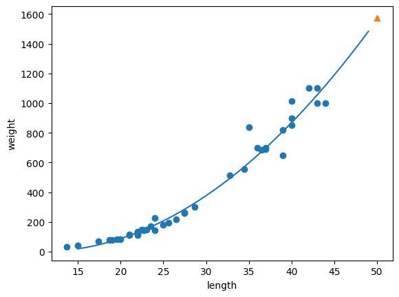
- 직선의 방정식이 아닌 곡선 또는 비선형 형태를 보이며, 이차항 이상의 값으로 변환해 선형회귀 성능을 향상
2) 2차항을 위한 브로드캐스팅
train_poly = np.column_stack((train_input ** 2, train_input))
test_poly = np.column_stack((test_input ** 2, test_input))
print(train_poly.shape, test_poly.shape)
(42, 2) (14, 2)
lr = LinearRegression()
lr.fit(train_poly, train_target)

print(lr.predict([[50**2, 50]]))
[1573.98423528]
print(lr.coef_, lr.intercept_)
[ 1.01433211 -21.55792498] 116.0502107827827
# 구간별 직선을 그리기 위해 15에서 49까지 정수 배열을 만듭니다
point = np.arange(15, 50)
# 훈련 세트의 산점도를 그립니다
plt.scatter(train_input, train_target)
# 15에서 49까지 2차 방정식 그래프를 그립니다
plt.plot(point, 1.01*point**2 - 21.6*point + 116.05)
# 50cm 농어 데이터
plt.scatter([50], [1574], marker='^')
plt.xlabel('length')
plt.ylabel('weight')
plt.show()
- 훈련 세트와 테스트 세트의 점수(결정계수, R^2)를 출력하면,
0.9706807451768623
0.9775935108325122
'데이터분석' 카테고리의 다른 글
| [23.07.21] 머신러닝(독버섯 찾기) - 36(2) (0) | 2023.07.21 |
|---|---|
| [23.07.21] 머신러닝(Random Forest) - 36(1) (0) | 2023.07.21 |
| [23.07.18] 머신러닝(k-최근접 이웃 회귀) - 33(2) (0) | 2023.07.18 |
| [23.07.18] 머신러닝(iris붓꽃데이터) - 33(1) (0) | 2023.07.18 |
| [23.07.17] 머신러닝(Machine Learning) - 32(1) (0) | 2023.07.18 |